Topic 2. Fluids dynamic

Introduction:

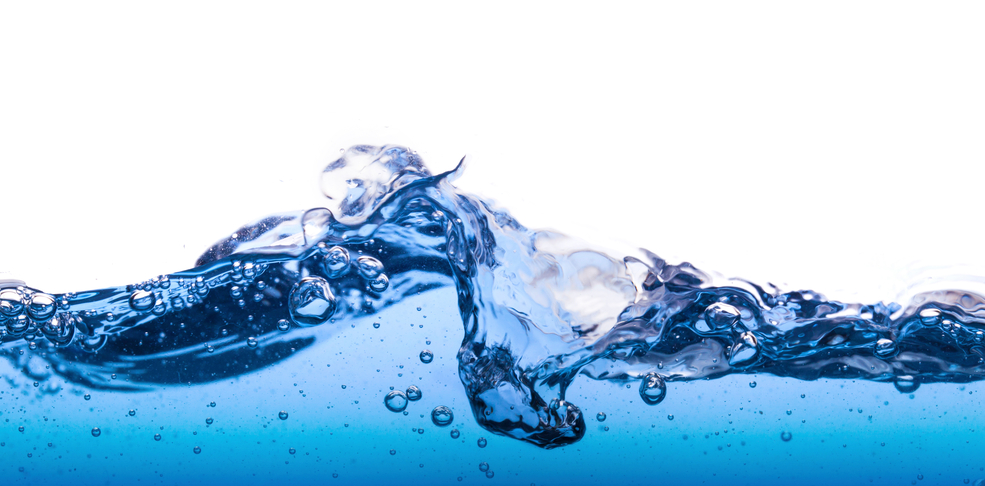
Figure 2.1 Fluid in motion

In the previous, topic you studied the properties of fluids at rest, going deep in the Archimedes and Pascal principles, as well as superficial tension and capillarity.

Now we are going to analyze the physics behind fluids in motion. The study of fluid dynamics can be very difficult, thus it is necessary to use an idealized model. This idealized model treats fluids as an ideal fluid. An ideal fluid is incompressible (can’t change its density by applying pressure) and non-viscous (no friction inside a fluid).

First, you will study the continuity equation, supposing that all fluids have a laminar flow. Them, you will go with the analysis of Bernoulli’s equation and non-ideal fluids.

---

Explanation:

2.1 Continuity equation

Laminar and Turbulent Flow

Figure 2.2 Laminar Flow

Figure 2.3 Turbulent Flow

When a fluid is in motion we can see two kinds of patterns: laminar and turbulent flow. Laminar flow presents when a fluid in motion continues in a stream line, all of the fluid’s molecules flow in the same direction (see figure 2.2). On the other hand, turbulent flow is when a fluid in motion swirls and doesn’t follow a single stream line (see figure 2.3).

Volume Flow Rate

To study motion of fluids is important to know the concept of volume flow rate. It refers to the volume of a fluid that passes through a closed conduit in a period of time. Mathematically, it is represented with the letter Q and it can be calculated by the following formula:

     (2.1)

Where:

Q= Volume flow rate (m3/s)
V= Volume (m3)
T= Time (s)

The volume flow rate can also be expressed in terms of the fluid’s speed (v, m/s) and the cross sectional area (A,m2) of the conduit:

     (2.2)

Using equation 2.1 and 2.2 the volume flow rate can be formally expressed as:

     (2.3)

Considering that when a fluid moves on a conduit its mass remains constant. Then it implies that the flow rate Q remains constant as well. Thus, we can make the next mathematical assumption:

     (2.4)

Replacing the equation 2.2 in 2.4, you will get an equation called continuity equation which applies for incompressible fluids:

     (2.5)

We can observe the continuity equation applied when you are watering the garden with a hose.

Let’s say you reduce the area of the hose by placing your finger in front of it. Then, according to the continuity equation the flow should stay the same. This means that to compensate for the loss in area, the speed needs to be larger.

  
Figure 2.4 Application of the continuity equation     

Indeed, when you place your finger in front of the water hose, the water will come out with a greater speed.

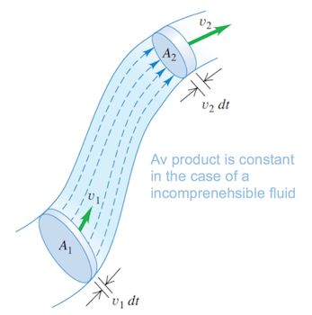
Figure 2.5 Flow tube with changing cross sectional area
Source: Sears, F. y Zemansky, M. (2013). Física universitaria con física moderna (13a ed.). México: Pearson/ Addison-Wesley.

To check an example, click here.

---

2.2 Bernoulli’s Equation

We know now that a fluid’s speed changes if the area at which is passing through changes. Similarly, the pressure a fluid in motion exerts will also change if there are variations in the height of a pipe.

In the eighteenth century, the scientist Daniel Bernoulli studied the conservation of energy of fluids that move through pipes and proposed a principle called after his name.

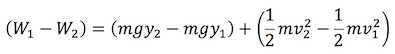
Work-energy theorem for fluids in motion

As we know, energy cannot be created or destroyed only transformed. Thus, a fluid in motion must conserve its energy but it will be transformed as it moves.

If you apply the work-energy theorem to two sections of a piping system where a fluid is passing, the following equation is obtained:

Potential energy U:

Kinetic energy K:

Since density  is the division of mass “m” by Volume V:

Mass can be expressed the following way:

Besides, work W is equal to the pressure p per the volume V:

The previous equations are equivalent to the following:

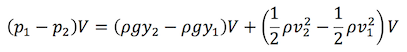
Canceling out volume V on both sides of the equation:

     (2.6)

Rearranging terms we get Bernoulli’s equation:

     (2.7)

In other words, the change in pressure of a fluid will be equal to the addition of the change in height (of the pipe) plus the change in speed (of the fluid). Bernoulli’s equation applies for ideal fluids.

The following figure displays this demonstration:

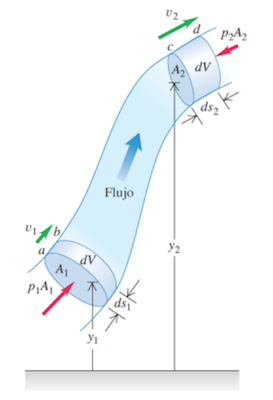
Figure 2.6 Demonstration of Bernoulli’s principle
Source: Sears, F. y Zemansky, M. (2013). Física universitaria con física moderna (13a Ed.). México: Pearson/ Addison-Wesley.

Torricelli’s Theorem

In the case of a liquid that flows under the effect of gravity, there is a simplification of Bernoulli’s equation called Torricelli’s theorem. Torricelli’s theorem is useful to calculate the speed at which a liquid will be moving, if there is no change in pressure and only the gravity acts on it. A good example of it is a hole on the wall of an open water tank. The pressure at the surface of the water and outside the tank is the same (the atmospheric pressure). Consequently, water will flow under the effect of gravity only.

Torricelli’s Theorem is then given by the following equation:

                 (2.8)

Where:

V= speed at which the liquid comes out of the tank
G= gravitational acceleration
H= height from the hole to the water’s surface

The speed at which the liquid will flow out of the water tank will be the same as an object free falling from the same height.

Example:

What is the speed of the water coming out from an opening of a full water tank of 5 m of height, if the cross sectional area of the opening is 0.0002 m²?

Solution:

The data given by the problem is:

h= 5 m
A= 0.0002 m2

Since we have an open water tank, we can use Torricelli’s theorem:

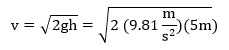
What is the water flow rate Q?

Now you have the necessary tools to calculate pressures, heights, piping diameters and fluid speeds applying the Bernoulli’s equation and the Torricelli’s theorem.

---

2.3 Non-Ideal Fluids

In the previous subtopic we assumed fluids were ideal, laminar and non-viscous. However, liquids aren’t always ideal. They have viscosity and some are turbulent when flowing.

Some examples of viscous fluids are the lava of a volcano, honey or blood. They flow slowly because they are viscous; another example is the engine oil, that is viscous when it’s cold, but when it is heated it flows easily through every duct of the motor.

 Another important concept of no ideal fluids, along viscosity, is turbulence.

When a fluid takes a small speed in a conduit, at the beginning the flow is laminar, very regular and predictable; however, if the speed is increased up to exceed a certain critical value, called Reynolds number, the flow changes, getting irregular and hard to predict.

A chaotic flow that changes with the time and is not stable is called turbulent flow.

For a flow to be whether laminar or turbulent depends on viscosity: less viscosity tends to a laminar flow. For example, if the flow of a waterfall could be restrained, the flow that seems turbulent will change to laminar. Knowing if a flow is laminar or turbulent may be done by using a dimensionless parameter that depends on the speed that the fluid takes, piping diameter, fluid viscosity, etcetera., it is called Reynolds number, and it is expressed as Re.

 If the piping the following limits are considered:

The turbulent flow is characterized then by random circular trajectories and the formation of whirlwinds. This flow is given to high speeds of flow and low viscosities of fluid.

---

Closure:

The river in the picture shows a turbulent flow. Turbulence is more common in nature, because there is more disturbance there than in a piping, where little obstructs the fluid circulation.

Bernoulli’s and Torricelli’s theorems as well as the continuity equation, have many applications in medicine, engineering, plumbing systems, aeronautics and hydroelectric generators.

Can you think of more applications? Read and do a small research about the applications of the physical principles you studied for this topic.

---

Bibliographic references:

• Sears, F. and Zemansky, M. (2013). Física universitaria con física moderna (13th ed.). México: Pearson/Addison-Wesley.  
• Young, H. and Freedman, R. (2004). Sear’s and Zemansky’s University Physics: with Modern Physics (11th ed.) United States: Pearson.
• Tippens, P. (2011). Física, conceptos y aplicaciones (7a ed.). México: McGraw-Hill.

---